H4. Rainfall Runoff Relationships

0 Comments catchment, GIS, GRASS, HEC-GeoHMS, HEC-HMS, hydrograph, modeling, Rainfall, Rainfall intensity, Rainfall Runoff Relationships, Runoff, TOPMODEL, Unit Hydrograph

Instructional Objectives

We will study the following at the conclusion of this lesson: 1. How hydrograph varies with catchment features
2. The relationship between hydrograph and rainfall properties
3. Unit Hydrograph: Definition, Assumptions, and Constraints
4. Using the Unit Hydrograph to Determine the Direct Runoff Hydrograph
5. Describe S-Curves and their uses.
6. Unit Hydrograph Derivation for Gauged Catchments
7. Unit Hydrograph estimation for ungauged catchments
8. Conceptual and empirically based rainfall-runoff models for catchments

Introduction

Previous Lesson was explained what a hydrograph is and that it indicates the response of water flow of a given catchment to a rainfall input. It is made up of runoff from various runoff phases, including base flow, interflow, and overland flow. Infiltration loss from the total rainfall hydrograph and base flow separation from it in order to produce the direct runoff hydrograph and effective rainfall hydrograph, respectively, have been explored. This lesson proposes to deal with the relationship between the effective rainfall over the catchment that causes the runoff and the direct runoff hydrograph of a catchment measured at a place (the catchment outlet).

We begin by going over how the various qualities of a catchment affect the hydrograph’s shape.

1. Hydrograph and the catchment’s characteristics

The catchment’s characteristics determine the hydrograph’s shape. The key elements are outlined below.

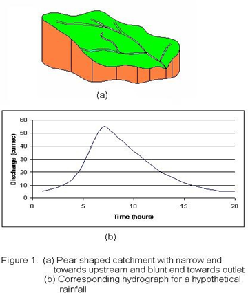
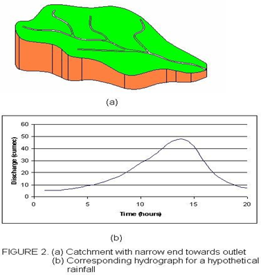
1.1 Shape of the catchment

A pear-shaped catchment has a fast-rising hydrograph with a concentrated high peak, while a catchment with a narrow end towards the outlet has a slow-rising hydrograph with a lower peak. Both catchments have the same volume of water, but the peak in the latter is attenuated.

1.2 Size of the catchment

The volume of runoff expected for rainfall is proportional to catchment size, but large catchments have significantly different response characteristics due to different phases of runoff. Non-linearity between rainfall and runoff becomes perceptible for smaller catchments, as shown by mathematical calculations.

1.3 Slope

The hydrograph’s shape is influenced by the slope of the mainstream cutting and valley sides. Larger slopes generate more velocity, displacing runoff faster. Smaller slopes store the balance over time, allowing gradual drainage. Two catchments with different slopes produce different hydrographs, with a flatter catchment producing a slow-rising moderated hydrograph.

2. Effect of rainfall intensity and duration on hydrograph

Isochrones, imaginary lines across catchments, explain how the duration of uniform rainfall affects the hydrograph’s shape. They indicate where water particles travel downward at the same time.

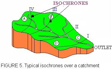
The hydrograph at the catchment outlet will continue to rise if the precipitation event begins at time zero, and after a time’t’ the flow from the isochrone I would have arrived at the catchment outlet. Thus, all of region A1 contributes to the outflow hydrograph after a time t pause.

By proceeding in this manner, it can be determined that, given the rain continues to fall for at least 4 time units (t), all catchment areas would be contributing to the catchment outflow. If the rain falls more, the hydrograph would plateau since it would not rise any higher.

3. Effect of spatial distribution of rainfall on hydrograph

The catchment image with the isochrones, as shown in Figure 6, can be used to describe the effect of the spatial distribution of rainfall, or the distribution in space. Assume that the areas between the isochrones experience varying quantities of precipitation (as indicated by the various blue hues in the illustration).

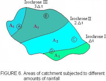
If it is presently believed that only area A1 receives rainfall but the other areas do not, Considering that this area is closest to the catchment outflow
, the generated hydrograph rises right away. If the rainfall continues for a time more than ‘Δt’, then the hydrograph would reach a saturation equal to re.A1, where re is the intensity of the effective rainfall.

Now suppose that constant intensity rain is only falling within
area A4, which is most remote from the catchment outlet. Since the lower boundary of A4 is the Isochrone III, there would be no resulting hydrograph till time ‘3Δt’.

If the rain continues beyond a time ‘4Δt’, then the hydrograph would reach a saturation level equal to re A4 where re is the effective rainfall intensity.

4. Direction of storm movement

The amount of the peak flow and the length of the hydrograph are both influenced by the storm’s movement in relation to how the catchments’ drainage network is oriented. The path of the storm has the biggest impact on elongated catchments because it tends to create lower peaks and a wider time base of surface runoff than storms that move downstream toward the catchment outlet. This is because, for an upstream moving storm, essentially little contribution from the lower watershed is present by the time the upper catchment contribution reaches the outlet.

5. Rainfall intensity

Rainfall intensity increases peak discharge and runoff volume for a given infiltration rate. In the initial storm, less intensity produces no surface runoff. As rain progresses, soil saturates and infiltration rates reduce. The relationship between rainfall intensity and discharge is not linear, but it may follow a linear relationship in catchment scales.

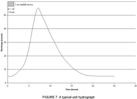
6. The Unit Hydrograph

A drainage basin’s unit hydrograph (abbreviated as UH) is described as the hydrograph of direct runoff that results from one unit of effective rainfall that is evenly distributed over the basin at a uniform rate during the designated time period known as unit time or unit duration. Effective rainfall is often measured in units of 1mm or 1cm, and the discharge ordinates are used to represent the outflow hydrograph. Depending on the size of the catchment and the features of the storm, the unit duration may be 1 hour, 2 hours, or 3 hours. The unit duration, however, cannot exceed the period of concentration, which is the amount of time it takes for the water to travel from the catchment’s farthest point to reach the outlet.

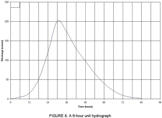
Figure 7 shows a typical unit hydrograph.

6.1 Unit hydrograph assumptions

When applying the unit hydrograph principle, the following presumptions are made:

1. Effective rainfall should be evenly distributed around the basin; in other words, if there are ‘N’ rain gauges evenly spaced throughout the basin, they should all record roughly the same quantity of precipitation during the designated time.

2. Throughout the unit period, the effective rainfall is consistent over the catchment.

3. Regardless of when an effective rainfall occurs, the direct runoff hydrograph for that catchment is always the same. Therefore, any earlier rainfall event is not taken into account. Due to its impact on the rate of soil infiltration, depressional and detention storage, and ultimately the resulting hydrograph, this preceding precipitation is also significant.

4. The unit hydrograph’s ordinates are inversely related to the effective rainfall hydrograph’s ordinate. As a result, if a 6-h unit hydrograph caused by 1 cm of rain is reported, a 6-h hydrograph caused by 2 cm of rain would simply signify that the unit hydrograph ordinates had doubled. As a result, the hydrograph’s base (from the beginning of ascent to the point at which discharge is zero) is unchanged.

6.2 Unit hydrograph limitations

The unit hydrograph theory is applicable to basins of any size, but its reliability diminishes beyond a 5000 sq. km catchment size. To meet the basic assumption, uniformly distributed storms producing rainfall excess are used, which rarely occur over large areas. When the basin area exceeds this limit, it is divided into sub-basins and the unit hydrograph is developed for each. Flood discharge at the basin outlet is estimated using flood routing procedures, which combine sub-basin floods along the river’s length.

7. Application of the unit hydrograph

Calculating direct runoff hydrograph in catchment for a given rainfall event is easy with a unit hydrograph. The effective rainfall hyetograph is obtained by deducting initial and infiltration losses from recorded rainfall, divided into T-hour duration blocks, and summed up to produce the total duration runoff.

8. Direct runoff calculations using unit hydrograph

The following table provides the ordinates of a 6-hour unit hydrograph (UH) of a catchment, and Figure 8 displays a comparable graphical depiction.

Time (hours)	Discharge (m³/s)
0	0
6	5
12	15
18	50
24	120
30	201
36	173
42	130
48	97
54	66
60	40
66	21
72	9
78	3.5
84	2

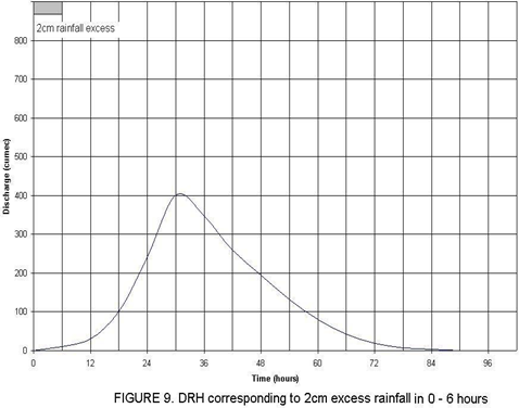
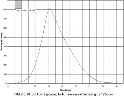
Assume further that the following table represents the effective rainfall hyetograph (ERH) for a certain storm in the area:

Time (hours)	Effective Rainfall (cm)
0	0
6	2
12	4
18	3

This indicates that 2 cm of extra rainfall was reported in the first six hours, 4 cm in the next six hours, and 3 cm in the following.

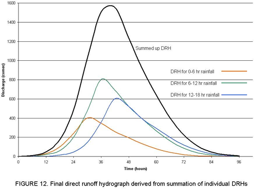
The three distinct hydrographs can then be used to determine the direct runoff hydrograph for the three surplus rainfalls by multiplying the hydrograph’s ordinates by the corresponding quantities of precipitation. The resulting DRH for each rainfall is suitably delayed by 6 hours because the 2 cm, 4 cm, and 3 cm of rainfall occur in consecutive 6-hour intervals.

The figures mentioned have examples of these.

DRH for 2cm excess rainfall in 0-6 hours

DRH for 4cm excess rainfall in 6-12 hours

DRH for 3cm excess rainfall in 12-18 hours

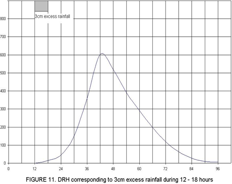
The three separate hydrographs are combined to create the final hydrograph, as seen in Figure 12.

A spreadsheet software like Microsoft Excel can be used to easily do the calculations needed to get the direct runoff hydrograph (DRH) from a given UH and ERH.

The following table contains a sample computation for the example that was graphically solved. Take note of the DRHs’ 6-hour shift in the second and succeeding hours.

Time (hours)	Unit Hydrograp h ordinates (m³/s)	Direct runoff due to 2 cm excess rainfall in the first 6 hours (m³/s) (I)	Direct runoff due to 4 cm excess rainfall in second 6 hours (m³/s) (II)	Direct runoff due to 3 cm excess rainfall in third 6 hours (m³/s) (III)	Direct runoff Hydrograph (m³/s) (I)+(II)+(III)
0	0	0	0	0	0
6	5	10	0	0	10
12	15	30	20	0	50
18	50	100	60	15	175
24	120	240	200	45	485
30	201	402	480	150	1032
36	173	346	804	360	1510
42	130	260	692	603	1555
48	97	194	520	519	1233
54	66	132	388	390	910
60	40	80	264	291	635
66	21	42	160	198	400
72	9	18	84	120	222
78	3.5	7	36	63	106
84	2	4	14	27	45
90		0	8	10.5	18.5
96		0	0	6	6

The coordinates of the DRH generated by the ERH are shown in the last column of the above table. The 6-hourly ordinates of the flood hydrograph should be obtained by adding the base flow to the DRH if it is known or predicted (Lesson 2.2).

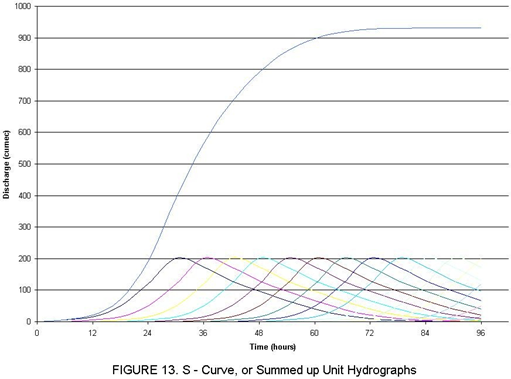
9. The S – curve

This idea applies to a fictitious storm with a 1 cm ERH and an endless duration that uniformly affects the entire catchment. This can be accomplished by repeatedly changing the UH by the T-duration. Due to the accumulation of an infinite number of T-hour unit hydrographs spaced T-hour apart, the final hydrograph (a typical one is depicted in Figure 13) is known as the S-hydrograph or the S-curve. The table below contains the necessary calculations for the example of the UH presented in the prior section.

Time	UH	UH Ordi- nates shifted	UH Ordi- nates shifted	UH Ordi- nates shifted	UH Ordi- nates shifted											Sum of all the UH
(hr)	Ordinates	by	by	by	by	…	…	…	…	…	…	…	…	…	…	… ordinates
		6 hr	12 hr	18 hr	24 hr
0	0	0	0	0	0	0	0	0	0	0	0	0	0	0	0	0	0
6	5	0	0	0	0	0	0	0	0	0	0	0	0	0	0	0	5
12	15	5	0	0	0	0	0	0	0	0	0	0	0	0	0	0	20
18	50	15	5	0	0	0	0	0	0	0	0	0	0	0	0	0	70
24	120	50	15	5	0	0	0	0	0	0	0	0	0	0	0	0	190
30	201	120	50	15	5	0	0	0	0	0	0	0	0	0	0	0	391
36	173	201	120	50	15	5	0	0	0	0	0	0	0	0	0	0	564
42	130	173	201	120	50	15	5	0	0	0	0	0	0	0	0	0	694
48	97	130	173	201	120	50	15	5	0	0	0	0	0	0	0	0	791
54	66	97	130	173	201	120	50	15	5	0	0	0	0	0	0	0	857
60	40	66	97	130	173	201	120	50	15	5	0	0	0	0	0	0	897
66	21	40	66	97	130	173	201	120	50	15	5	0	0	0	0	0	918
72	9	21	40	66	97	130	173	201	120	50	15	5	0	0	0	0	927
78	3.5	9	21	40	66	97	130	173	201	120	50	15	5	0	0	0	930.5
84	2	3.5	9	21	40	66	97	130	173	201	120	50	15	5	0	0	932.5
90	0	2	3.5	9	21	40	66	97	130	173	201	120	50	15	5	0	932.5
96	0	0	2	3.5	9	21	40	66	97	130	173	201	120	50	15	5	932.5

The equilibrium discharge is provided as (A /T)*104 (m3/h), where A is the average effective rainfall intensity, and 1/T (mm/h) is the average effective rainfall intensity that produces the S-curve.

The catchment area is measured in km2, and the unit hydrograph time is measured in hours.

10. Application of the S – curve

Despite being a theoretical idea, the S-curve can be used to accurately calculate a t-hour UH from a T-hour UH where t is less than T or greater than T but not exactly a multiple of T. If t is a multiple of T, the appropriate UH can be calculated without an S-hydrograph by adding the necessary number of UH that have been consecutively lagged behind by T-hours.

In all other situations, add t hours to the original S-hydrograph that was obtained for the T-hour UH to get a lagged S-hydrograph. To create the t-hour graph, subtract the ordinates of the second curve from the first. Then, scale the discharge hydrograph’s ordinates by a factor of t/T to get the actual t-hour UH that would be produced by a total of 1 cm of rainfall over the watershed. The S-curve derived in the previous section serves as an illustration for this.

Remember that a 6-hour UH was used to produce the S-curve. Let’s calculate the UH for a three-hour period. We interpolate and write the ordinates of the S-curve at each 3-hour interval because we don’t know them, as shown in the table below:

Time	S-curve ordinates as derived from 6-hr UH (I)	S-curve ordinates as derived from 6-hr UH but with inter- polated values (II)	S-curve ordinates as derived from 6-hr UH lagged by 3 hrs. (III)	Difference of the two S- curves (II) – (III) (IV)	3-hr UH ordinates Col. (IV) divided by (3hr/6hr) = (IV)*2
(hours)	(m³/s)	(m³/s)	(m³/s)	(m³/s)	(m³/s)

0	0	0		0
3		2.5	0	2.5
6	5	5	2.5	2.5
9		12.5	5	7.5
12	20	20	12.5	7.5
15		45	20	25
18	70	70	45	25
21		130	70	60
24	190	190	130	60
27		290.5	190	100.5
30	391	391	290.5	100.5

33		477.5	391	86.5
36	564	564	477.5	86.5
39		629	564	65
42	694	694	629	65
45		742.5	694	48.5
48	791	791	742.5	48.5
51		824	791	33
54	857	857	824	33
57		877	857	20
60	897	897	877	20
63		907.5	897	10.5
66	918	918	907.5	10.5
69		922.5	918	4.5
72	927	927	922.5	4.5
75		928.75	927	1.75
78	930.5	930.5	928.75	1.75
81		931.35	930.5	0.85
84	932.5	932.5	931.35	1.15
87		932.5	932.5	0
90	932.5	932.5	932.5	0
93		932.5	932.5	0
96	932.5	932.5	932.5	0

11. Derivation of unit hydrograph

An observed flood hydrograph at a streamflow gauging station may be owing to a complicated rainfall event with varied intensities, or it may be the consequence of an isolated severe short-duration storm with virtually uniform distribution in time and place. In the first scenario, the observed hydrograph would typically be single peaked, however in the second scenario, depending on the variation in rainfall intensities, the hydrograph could be multi peaked. For the sake of this course, we will just assume that rainfall is more or less equally distributed in time and space in order to illustrate how the unit hydrograph is derived. The steps of the process can be broadly categorized as follows:

1. To ensure that the volume and distribution of rainfall over the watershed are precisely known, obtain as many rainfall records for the research region as you can. Only storms that are singular occurrences with a consistent spatial and temporal distribution are chosen, coupled with the hydrograph that was observed at the watershed outlet point.

2. Out of the uniform storms data gathered in Step 1, storms fitting the following characteristics are typically preferred and chosen.

3. Storms that produce rainfall for 20 to 30 percent of the basin lag,

4. Storms with an excess of 1 to 4.5 cm of rain.

5. Separate the base flow (explained in lecture 2.2) from the observed total flood hydrograph for each storm, and then plot the direct runoff hydrograph.

6. Calculate the area under the DRH curve to get the total amount of water that has passed the flow measuring point. Divide the volume of flow (step 3) by the catchment area to determine the average uniform rainfall depth that produced the DRH because the area of the watershed under consideration is known. This provides the storm-related effective rainfall (ER). To obtain the appropriate ERs, this process must be done for each selected storm.

7. Indicate the hydrograph ordinate for each storm at T hours, where T is the hourly length of rain. To get the UH for each storm, divide each ordinate in the hydrograph by the associated storm ER.

8. Using the S-curve approach, all UHs collected from various storm events should be brought to the same duration.

9. By averaging the ordinates of the several UH produced in step 6, the final UH of a specified duration is obtained.

12. Unit hydrograph for ungauged catchments

The Central Water Commission recommends using Flood Estimation Reports for generating synthetic unit hydrographs for catchments with insufficient rainfall or concurrent runoff data. These hydrographs are constructed from basin characteristics, and the design flood is estimated by applying the design storm rainfall to the hydrograph developed using these reports.

13. Catchment modeling

With the availability of personal computers, numerical modeling of catchment dynamics and simulation has become more prevalent. Conceptual mathematical models represent physical processes by equations, which are solved using computer language. Users input data through a Graphical User Interface (GUI) and now use Geographic Information System (GIS) software for spatial information interaction. Output results are displayed graphically.

• http://www.nrc.gov/reading-rm/doc- collections/nuregs/contract/cr6656/cr6656.pdf
• www.hydrocomp.com/simoverview.html
• http://www.ems- i.com/gmshelp/numerical_models/modflow/modflow_conceptual_m odel/the_conceptual_model_approach.htm

14. Examples of catchment models

Many models, developed by academic institutions and government agencies, are free and available for non-commercial download on the internet, although many are sold commercially.

• US Army corps of Engineers’ HEC-HMS and HEC-GeoHMS
• US Army corps of Engineers’ GRASS
• US Army corps of Engineers’ TOPMODEL

IIT Kharagpur’s Department of Civil Engineering has created a deterministic watershed simulation model, which can be accessed for educational purposes upon request.

15. Important terms

1. Linearity: A relationship between rainfall and runoff from a catchment that is linear shows that changes in runoff from the catchment’s outlet are connected to changes in rainfall across the catchment as a whole.

2. Basin lag: The interval between the peak flow and the center of rainfall is known as the basin lag.

3. Graphical User Interface (GUI): A GUI is an interface that uses graphical images to represent programs, files, and settings. Icons, menus, and dialog boxes can all be examples of these pictures. By using a mouse or keyboard to point and click, the user picks and activates these options. A certain GUI component, like a scroll bar, functions uniformly across all programs.

4. Geographic Information System (GIS): A system for the entry, storage, retrieval, analysis, and display of interpreted geographic data. GIS systems are typically computer-based. The database is often made up of geographical representations that resemble maps, sometimes known as coverages or layers. A three-dimensional matrix of time, place, attribute, or action may be present in these levels. Any other related or derived geographic data may also be included in a GIS, such as digital line graph (DLG) data, digital elevation models (DEM), geographic names, land-use characterizations, land ownership, land cover, registered satellite and/or areal photography, and so on.

5. HEC-HMS: The Dendritic Watershed Systems Precipitation-Runoff Processes of the Hydrologic Modeling System (HEC-HMS) are Simulated. It is intended to be useful in a broad range of geographic contexts for addressing the broadest range of issues. This encompasses runoff from local urban or natural watersheds, big river basin water supply, and flood hydrology. For studies of water availability, urban drainage, flow forecasting, the influence of future urbanization, reservoir spillway design, flood damage mitigation, floodplain regulation, and system operation, hydrographs generated by the program are used either alone or in conjunction with other software.

6. HEC-GeoHMS is a software package for ArcView Geographic Information System that uses digital terrain information to create hydrologic modeling inputs. It transforms drainage paths and boundaries into hydrologic data structures, develops grid-based data, and creates watershed and stream characteristics.

7. GRASS: GRASS is a collection of integrated software tools that enable users to create maps and perform image processing, digitizing, and geographic information system functions. GRASS is open-source software with freely downloadable C source code.

8. TOPMODEL: Based on time series of precipitation and evapotranspiration as well as topography data, TOPMODEL forecasts catchment water discharge and spatial soil water saturation pattern.

References

• Subramanya, K (2000) Engineering Hydrology, Tata Mc Graw Hill
• Mutreja, K N (1995) Applied Hydrology, Tata Mc Graw Hill