Precipitation refers to water falling from the atmosphere to Earth’s surface.

Instructional Goals

After finishing this lesson, the learner will understand:

1. The role of precipitation and evapotranspiration in the hydrologic cycle.
2. The factors that cause precipitation.
3. The means of measuring rainfall.
4. The way rain varies in time and space.
5. The methods to calculate average rainfall over an area.
6. What are Depth – Area – Duration curves.
7. What are the Intensity – Duration – Frequency curves.
8. The causes of anomalous rainfall record and its connective measures.
9. What are Probable Maximum Precipitation (PMP) and Standard Project Storm (SPS).
10. What is Actual and Potential evapotranspiration.
11. How can direct measurement of evapotranspiration be made.
12. How can evapotranspiration be estimated based on climatological data.

1. Causes of precipitation

Cloud formation requires moist air to cool, condensing through adiabatic cooling and elevation, resulting in various precipitation types:

• Frontal precipitation
Precipitation occurs from air expansion on ascent near frontal surface.
• Convective precipitation
Precipitation occurs when warmer air moves upward, causing showery, rapid precipitation.
• Orographic precipitation
Air masses hit mountain barriers, causing precipitation and condensation, with windward side receiving the most precipitation and leaveward side receiving less.

Quantifying rainfall is crucial for water resources engineering and obtaining analytical information.

2. Regional rainfall characteristics

Rainfall in a region is not uniformly distributed or constant over time. It is difficult to predict when and how much rain will fall, but measuring the amount at any point provides an idea of the rainfall pattern within an area.

3. Measurement of rainfall

Rainfall depth can be measured using a measuring cylinder with a length scale, typically in mm. This method ensures uniform distribution of rainfall over an area, rather than a single depth. Standard-sized measuring cylinders are used for spatial variation, while recording rain-gauges are used for time-varying variations. Radars, developed using modern technology, measure rainfall over an entire region but are more costly than conventional methods.

4. Variation of rainfall

Rainfall measurement estimates water falling over land, infiltrating soil and flowing to streams or rivers. A scientific study studies the hydrologic cycle by examining the correlation between catchment water, groundwater addition, and streamflow. Some water evaporates or is extracted by plants.

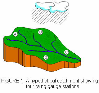
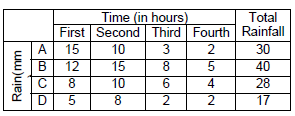
In Figure 1, Four rain gauges are used to depict a river’s catchment, and a table with an estimated recorded value of rainfall depth for each gauge is included.

Estimating average rainfall over catchments using discrete measurements and three commonly used methods.

5. Average rainfall depth

Rainfall record time for non-recording gauges ranges from 1 minute to 1 day, while recording gauges continuously record rainfall from 1 day to 1 week. Average depth of rainfall over catchments can be found using three methods:

• The Arithmetic Mean Method
• The Thiessen Polygon Method
• The Isohyetal Method

Arithmetic Mean Method

The Arithmetic Mean Method, which averages all rainfall depths as indicated in Figure 2, is the most straightforward of all.

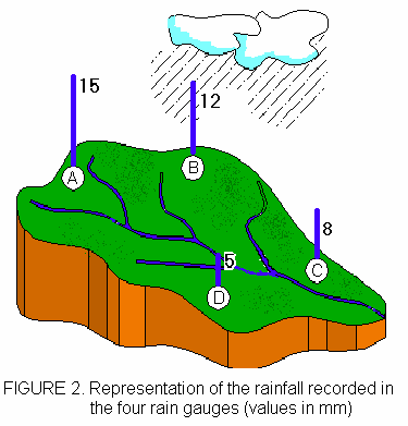
The following chart shows the average rainfall as the arithmetic mean of all the data from the four rain gauges:

(15 + 12 + 8 + 5 )/4 = 10.0 mm

The Theissen polygon method

This approach, which Thiessen first suggested in 1911, takes into account the representative region for each rain gauge. These might alternatively be regarded as each rain gauge’s effect zones, as depicted in Figure 3.

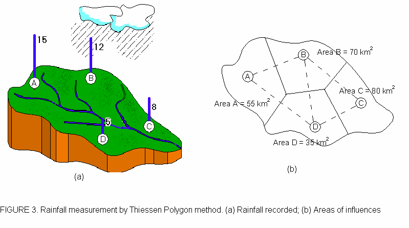
The following three phases make up a strategy for locating these areas:

1. forming triangles by connecting the sites of the rain gauge stations in a straight line.

2. The so-called “Thiessen polygons” are created by dividing the triangles’ edges in half.

3. To determine the region of influence corresponding to each rain gauge station, calculate the area bordered by the polygon edges and the catchment boundary (if applicable).

The “weighted” average rainfall over the catchment for the example given is calculated as,

(65 x 15 + 70 x 12 + 35 x 8 + 80 x 5)/(55 + 70 + 35 + 80) = 10.40 mm

The Isohyetal method

This is one of the procedures that is thought to be the most accurate, but it is subject to the knowledge and expertise of the analyst. In order to use the method, isohyets must be plotted as shown in the image, and enclosed areas must be calculated between isohyets or between an isohyet and the catchment boundary. If the catchment map is produced to a scale, the areas can be measured using a planimeter.

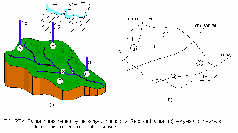
The regions contained between two consecutive isohyets for the issue depicted in Figure 4 may be considered to be as follows and are calculated as follows:

Area I is 40 km2.

Area II is 80 km2.

Area III is 70 km2.

Area IV is 50 km2.

240 km2 is the total catchment area.

Areas II and III are separated by two isohyets. Consequently, the following rainfall depths may be thought of as correlating to these areas:

Area II: corresponding to a rainfall depth of (12.5 mm x (10 + 15)/2).

Area III: corresponding to a rainfall depth of 7.5 mm (5 + 10)/2.

Although there is no record, a rainfall depth of 15mm is accepted for Area I even though we would anticipate more rainfall to fall there than that. Similar calculations must be made for Area IV’s 5 mm of rainfall.

As a result, the isohyetal technique determines that the average amount of precipitation is

40 x 15, 80 x 12, 70 x 7.5, and 50 x 5 divided by 240 equals 9.89 mm.

Please be aware of the terminology used in this section.

Isohyets: Map lines that travel through locations with the same amount of rainfall observed there during the same time period (these lines are generated after taking the local topography into account).

Planimeter: This drafting tool is used to calculate the size of a planar region that is graphically represented.

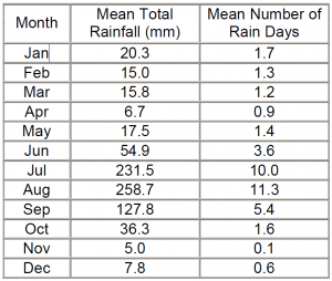
6. Mean rainfall

Mean annual rainfall is determined by averaging consecutive years’ total rainfall, while mean monthly rainfall is determined by averaging monthly total rainfall for several consecutive years. A record number of years is required for accurate estimates.

Rainfall and rainy days in New Delhi are provided by WMO:

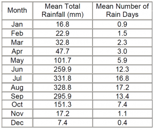
Kolkata’s comparison with similar source:

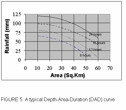
7. Depth-Area-Duration curves

Designing water resource structures requires understanding rainfall areal spread within the watershed and the expected high rainfall. Storm events often start with heavy downpours and gradually reduce over time, making rainfall depth not proportional to observation duration. Large areas may have less average rainfall due to variations in rainfall. a Depth-Area-Duration (DAD) analysis is used to determine the optimal areal precipitation for different durations and extents.

DAD analysis results in DAD curves, depicted in Figure 5.

8. Intensity-Duration-Frequency curves

Continuous rainfall events analysis involves evaluating intensities using part storm records and presenting them in graphical form.

Here, we introduce two novel ideas, namely:

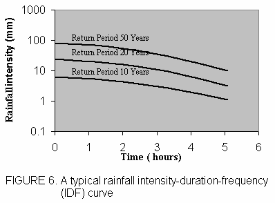
• Rainfall intensity:

Rainfall event recorded at a station divided by time, counting from beginning.

• Return period

This is the period of time following which a storm of a particular magnitude is likely to occur again. This is discovered by reviewing historical rainfall data from numerous incidents that were recorded at a station. The return period is inversely related to the frequency of the rainfall event, also known as the storm event. This sum is frequently stated as a percentage by multiplying it by 100. The number of times the given occurrence may be anticipated to be equaled or exceeded in a 100-year period is the frequency (represented as a percentage) of rainfall of a certain magnitude.

9. Analysis of anomalous rainfall records

Regularly monitor rainfall recorded at rain gauges within a catchment for anomalies. Some gauges may stop functioning, causing a different trend from past data. These anomalies can be caused by neighborhood or ecosystem changes, and can be classified as major or minor.

• Missing rainfall record
• Inconsistency in rainfall record

 

Missing rainfall record

Rainfall records may be discontinued due to operational reasons. Approximating missing records using the Normal Ratio Method using three nearby stations.

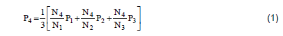
N1, N2, N3, and N4 are the four stations’ average yearly precipitation, P1, P2, and P3 are the rainfall totals recorded at stations 1, 2, and 3, respectively, and P4 is the precipitation at the missing location.

 

Inconsistency in rainfall record

Consistency check for rainfall records involves comparing accumulated annual precipitation of suspected stations with standard or reference stations using a double mass curve, assessing changes in gauge location, exposure, or instrument.

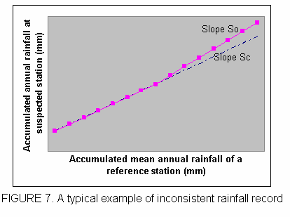
We may write the computed slopes S0 and Sc from the graphed line

where Pc and P0 are the original and corrected rainfall measurements made at the suspected station at any given period. The double mass curve’s original and corrected slopes are denoted as Sc and S0.

10 Probable extreme rainfall events

In terms of water resources engineering, two characteristics of extreme rainfall occurrences are crucial. Which are:

Probable Maximum Precipitation (PMP)

The PMP is the maximum rainfall over a region, calculated by maximizing storms for critical atmospheric conditions. It varies across the Earth’s surface and varies within India, with higher PMP in hot, humid equatorial regions and humid regions in the South Meghalaya plateau.

Standard Project Storm (SPS)

This storm is the heaviest rainstorm in the basin, occurring during rainfall records and not maximized for critical conditions but potentially transposed from an adjacent region.

The ways to earn PMP and SPS are complicated, but the interested reader can get assistance in hydrological textbooks by consulting the ones listed below:

• Mutreja, K N (1995) Applied Hydrology, Tata McGraw Hill
• Subramanya, K (2002) Engineering Hydrology, Tata McGraw Hill